State Space Models: How Control Theory can echo Machine Learning

I wrote in a previous post how transformers are kind of like system identification methods applied to some sequence in a state space. In this post we try to understand if the other way round is true.

We already saw previously ¹ how predicting words/tokens is a sequence to sequence mapping problem, which is the subject of a lot of prediction, estimation, and controls problems. In fact, we leveraged a transformer’s sequence mapping ability and applied it to a controls problem of trajectory prediction for a simple 2D car model ¹. Can we do the other way round? Turns out: yes we can!

To understand this link, let us do a quick revision to linear dynamical systems. Let us go back to a simple linear time invariant system of the form $$\dot{x}(t)=Ax(t) + Bu(t)$$ (Typically matrices, $$A$$ can be an operator on a finite dimensional space $$\mathcal{X}$$ and $$B$$ from $$\mathcal{U}$$ into $$\mathcal{X}$$). A typical control synthesis problem concern with the following: Find a control sequence $$u$$ (typically a sequence/signal over time that is $$L^2([t_0,t_1],\mathcal{U}))$$ such that one can drive $$x(t_0)=x_0$$ can be driven to some other $$x(t_1)=x_1$$ under the dynamics $$A,B$$. So the control problem is to find $$u(t)$$ over $$[t_0,t_1]$$ to drive the system’s state from $$x_0$$ to $$x_1$$. The differential state dynamics can be solved as:

$$x(t_1)-e^{At_1x_0}=\int^{t_1}_{0} {e^{A(t_1-\tau)} Bu(\tau)}d\tau$$

To answer the question of what such a control sequence $$u^*$$ would look like is fairly nuanced (at least in continuous time) ². However, before jumping to finding the answer, a fair initial query concerns when can we find such a solution?

We can look at the sequence map of $$x_1$$ under the linear operator $$Tu=\int^{t_1}_{0} {e^{A(t_1-\tau)} Bu(\tau)}d\tau$$. It is no coincidence that this operator is a convolution on $$u$$. Skipping some technical details (that can be found in Chapter 5 of ²), turns out that one can find the sequence $$u$$ getting mapped as $$Tu$$ if (and only if) for an arbitrary $$x_0,x_1$$, one can solve $$x(t_1)-e^{At_1x_0}=Tu$$, or the range of the operator $$T$$ spans the entire state space $$\mathcal{X}$$. This property is often called controllability.

Alternatively, $$\mathrm{range}(T)$$ is often smaller than $$\mathcal{X}$$; or, there is a smaller dimensional state space that is controllable. Since the underlying systems are all linear, the controllable part of the state space is found by the range of the matrix $$W_c=[B \,AB\, \cdots \, A^{n-1}B]$$. This matrix $$W_c$$ is called the controllability matrix.

In essence, under linear dynamics, the sates that you can “hit” with the matrices $$A,B$$ is given by the range of $$W_c$$. Additionally, often times we do not observe $$x$$ itself, but some mapping of it, say, $$y(t)=Cx(t)$$. Then, the input sequence is some $$u[t_0,t_1]$$ is getting mapped to the output sequence $$y[t_0,t_1]$$ – and if we closely observe, the output sequence is a convolution as the figure below:

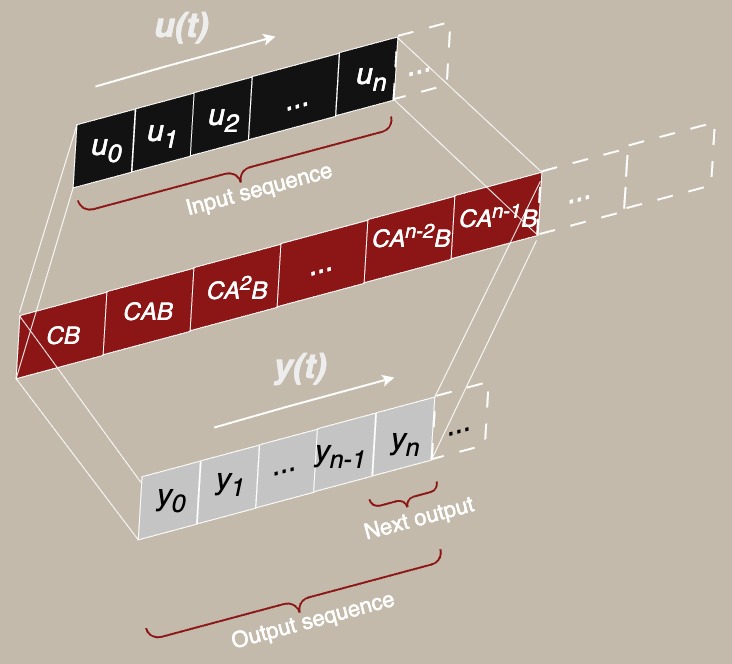
This is where things finally start to add up. State space models (SSMs) inspired from the control problems above have been gaining a lot of traction for sequence modeling lately (see Mamba, and all its derivatives ³⁴). By parameterizing the controllability convolution kernel via its state space matrices $$A,B,C$$, SSMs can often efficiently model long-range dependencies with relatively fewer parameters than attention-based methods. In this way, SSMs attempt to describe the input-output sequences $$u(t), y(t)$$, by first projecting to a higher dimensional feature/hidden space $$\mathcal{X}$$, and the output sequence map is a learnable controllability convolution kernel $$W_c$$. In some flavors such as S4, this is exactly the fixed kernel $$W_c$$, while in more sophisticated selective state space methods like Mamba, it is a time-dependent kernel $$W_{c}(t)$$. The key idea is the same: to predict the sequence as $$y = W_c * u$$ as a learnable sequence-to-sequence map in the state space.

Just like the previous post, where we had a tiny transformer and applied it to a state space/controls problem of system identification for a 2D car ⁵, now we try the dual problem: a tiny mamba SSM to try to do a token sequence prediction task :)

 1
 2
 3
 4
 5
 6
 7
 8
 9
10
11
12
13
14
15
16
17
18
19
20
21
22
23
24
25
26
27
28
29
30
31
32

class SSMLayer(nn.Module):
   def __init__(self, n_state, n_in, vocab_size):
       super().__init__()
       self.n_state = n_state
       self.A = nn.Parameter(torch.randn(n_state, n_state) * 0.1)
       self.B = nn.Parameter(torch.randn(n_state, n_in) * 0.1)
       self.C = nn.Parameter(torch.randn(vocab_size, n_state) * 0.1)
       self.D = nn.Parameter(torch.randn(vocab_size, n_in) * 0.1)
       self.state_norm = nn.LayerNorm(n_state)

   def forward(self, u_emb):
       B, T, n_in = u_emb.shape
       x = torch.zeros(B, self.n_state, device=u_emb.device)
       logits = []
       for t in range(T):
           u_t = u_emb[:, t, :]
           x = torch.tanh(x @ self.A.T + u_t @ self.B.T)
           x = self.state_norm(x)
           y_t = x @ self.C.T + u_t @ self.D.T
           logits.append(y_t)
       return torch.stack(logits, dim=1)

class TinyMamba(nn.Module):
   def __init__(self, vocab_size, n_embed=128, n_state=128):
       super().__init__()
       self.embed = nn.Embedding(vocab_size, n_embed)
       self.ssm = SSMLayer(n_state, n_embed, vocab_size)
   
   def forward(self, x):
       emb = self.embed(x)
       logits = self.ssm(emb)
       return logits  

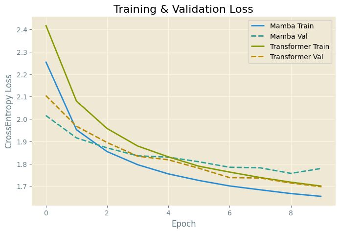
The complete code for this post can be found here ⁶. Here I train both models on a tiny fraction of wikitext to try to train them to learn next token prediction task on a cross entropy loss. While both models are really small, trained over a tiny dataset, with relatively few parameters, a few things can still be inferred. For instance, the tiny mamba takes about half the time per epoch to train.

Training Mamba...
Epoch 1: train_loss=2.2565, val_loss=2.0158, time taken=62.5461s
...
Training Transformer...
Epoch 1: train_loss=2.4196, val_loss=2.1047, time taken=117.1591s
...

Additionally, both models seem to have a similar cross entropy loss in train, as well as validation datasets.

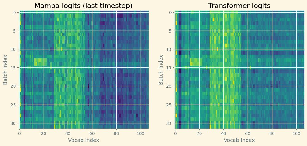
As far as their next token prediction is concerned, tiny mamba and tiny transformer have 28864 and 115819 trainable parameters, respectively. And when trained on 1% of the wikitext dataset, and presented with the input prompt: “control theory is a field of ”, here is what both models have to say:

tiny mamba: the season , the season , the season , the season
tiny transformer: team 's state the state the season , and the state

While the tiny mamba and tiny transformer both predict gibberish, both are equally confused as seen in comparing the logits directly! That is, state space models can provide comparable performance to transformers on sequence to sequence tasks, with a much smaller number of parameters. In fact, SSMs are often preferred in literature over transformers in certain tasks with long-range prediction or memory requirements ⁴. Note that for my particular training parameters, the SSM did slightly better in training, but worse in validation. SSMs are methods of choice for short to medium range sequence modeling tasks.

This post’s aim was not to capture benefits or any particular sequence to sequence modeling method over a different one. Instead, this is a continuation of my ongoing side-quest of finding applications from one field (typically controls engineering), into other different fields. If you liked this post, a much more profound result awaits here ³ where the inventors of mamba determine how transformer models and state space models are closely related.

> Written with StackEdit.