Why are Gaussian distributions present Everywhere?

Well, if one were to cut to the chase, it appears to be because of the Central Limit Theorem (CLT). However, there is more underlying structure under the hood as to why the Gaussians seem to be the ‘chosen’ distributions. In this post we will go through some in-depth analysis beyond the typical textbook to try to get some juice worth the squeeze. And hopefully it would demystify the ubiquity – from statistics, to thermodynamics, to measurement errors – of Gauss’s eponymous distributions. To this end, this write up is a shallow dive into Gaussian ubiquity from a few different angles.

Let’s revisit the definition of a moment generating function (MGF) for a random variable $$X$$ with a cumulative distribution function $$F_X(x)$$ as $$M_X(t) =\int_{-\infty}^\infty {e^{tX}dF_X(x)} = \mathbb{E}[e^{tX}]$$. The so-called “generating” property is a result of the Taylor expansion of $$e^{tX}=\sum_{n=0}^\infty \frac{(tX)^n}{n!}$$. Since expectation is a linear operator, the $$n$$-th moment $$m_n=\mathbb{E}[X^n]$$ is given by the $$n$$-th derivative of the MGF evaluated at 0. Two important properties of the MGF are:

1. MGF of $$X$$ is the two-sided Laplace transform of the probability density function of $$X$$ evaluated at $$-t$$, and
2. For independent random variables, the MGF of their sum is the product of their MGFs (i.e., $$M_{X+Y}(t)=M_X(t)M_Y(t)$$).

Even though the resulting moments are useful, they are a little nasty to deal with, especially when dealing with sums of random variables. This is where the cumulant generating function (CGF) comes in, defined as the logarithm of the MGF: $$K_X(t)=\log{M_X(t)}=\sum^\infty_{n=1}\frac{\kappa_n}{n!}t^n$$. The coefficients $$\kappa_n$$ are the cumulants of $$X$$, recovered similar to moments by evaluating the $$n$$-th derivative of the CGF at 0. Note that for a Gaussian distribution, the first cumulant equals the distribution mean, second cumulant equals its variance, and all higher cumulants are zero ¹. This must be noted as a key test for Gaussianity.

1. So the MGF is the logarithm of the Fourier transform of the probability density function, and
2. For independent random variables, the cumulants of their sum is the sum of their cumulants (i.e., $$\kappa_n(X+Y)=\kappa_n(X)+\kappa_n(Y)$$).

These important properties of the MGF and CGF are good to remember (and maybe even derive by yourself!). While both CGF and MGF are not useful by themselves, they are tools to “generate” moments and cumulants – which are useful in analyzing distributions. The result of additivity of independent cumulants is far more consequential: cumulants scale under homogeneous transformations.

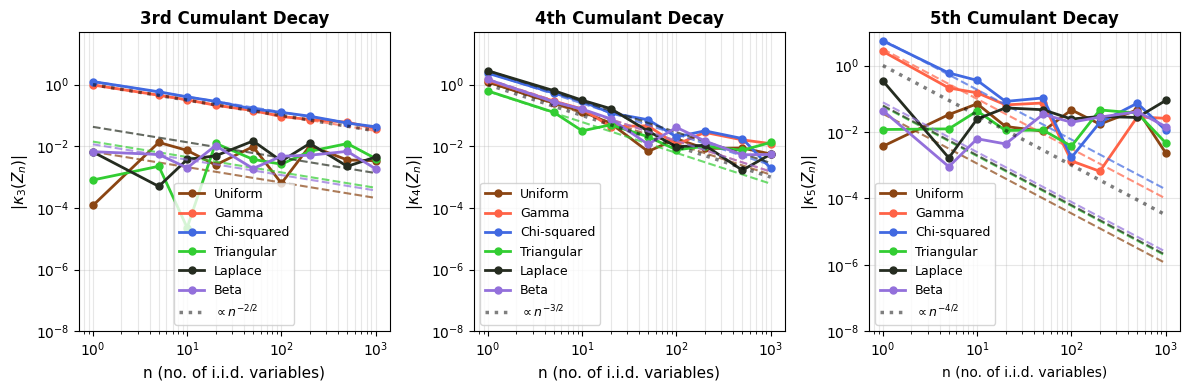
That is, summing $$n$$ independent identically distributed (i.i.d.) variables scales the resulting cumulant linearly: $$\kappa_r(X_1+...+X_n)=n\kappa_r(X)$$. And $$\kappa_r(cX)=c^r \kappa_r(X)$$. Let us look at what this means for $$n$$ i.i.d. random variables. Let the sample mean be $$\mu=\mathbb{E}[X_i]$$, and sample variance $$Var(X_i)=\sigma^2$$, and let $$S_n$$ denote the sum of the $$n$$- random variables. If we want to analyze the limiting tendencies of $$S_n$$, we need to prevent the probability mass from spreading unbounded to infinity, which can be done be redefining a normalized variable: $$Z_n=\frac{S_n-n\mu}{\sigma\sqrt{n}}$$ such that the rescaled variable s zero mean and unit variance via due to our construction. In order to understand the distributions of $$Z_n$$, it helps to analyze its cumulants. If the original cumulants are $$k_r=\kappa_r(X)$$, then due to the additivity property of cumulants, we have $$\kappa_r(S_n)=n\kappa_r(X)=nk_r$$. Centering around 0, we get: $$\kappa_1(S_n-n\mu)=n\mu-n\mu=0$$, and $$\kappa_r(S_n-n\mu)=\kappa_r(S_n)=nk_r$$ for $$r\geq2$$. Finally scaling by the constant $$\frac{1}{\sigma\sqrt{n}}$$, we get: $$\kappa_r(Z_n)=\frac{1}{\sigma^r n^{r/2}} (nk_r)=\frac{k_r}{\sigma^r}n^{1-r/2}$$.

The interesting thing to note here in the limiting case is that for $$r=1$$, the mean for $$Z_n$$ goes exactly to 0. Similarly, the Variance for $$r=1$$ goes exactly to unity. So far we are good. But a by-product of additivity and homogeneity of cumulants is that all higher cumulants tend to 0 as $$n$$ increases! Note that this means Gaussian distributions emerge out of i.i.d. sums as a natural byproduct. That is, Gaussians are “universal attractors” of i.i.d. random variables as Gaussian is the only distribution that contains quadratic information. As a result, Gaussian distributions are found everywhere, especially in large scale properties, as Gaussian cumulants are fixed points for large scale behaviors. When many individual (microscopic) properties are combined to fewer effective (macroscopic) properties, the way the resulting cumulants are shaped tell us about the macroscopic properties that survive, and the ones that get destroyed. As higher order cumulants scale with a higher power of microscopic contributors, they decay faster when renormalized. The effective macroscopic descriptors remaining in the limiting case are only the mean and the variance.

That is, homogeneous scaling of cumulants encodes how the underlying distribution’s complexity in large-scale systems collapses, and Gaussians emerge as a stable fixed-point under this coarse-graining.

Two Examples:

The (higher order) cumulant decay property, and CLT are good checks for Gaussian distributions in random variables. We check for this universal attractor property of Gaussian distributions by checking six different distributions: Uniform, Gamma, Chi-squared, Laplace, Beta, and Triangular distributions, summed over $$10^5$$ data points. Comparing cumulants, we do observe higher order cumulants decaying, no matter which distribution we sample the random variables from, though at different rates for different distributions². So no matter which distribution you start from, the sums do gravitate towards Gaussians, shown below. This not only enables parametric testing (like t-tests), even when the underlying data are not Gaussian, but also allows for confidence interval-based testing to estimate where population means may lie.

If you are thinking this foundational property would have further implications in statistical machine learning, you are correct.

The weighted sum after a linear layer $$W^Tx+b$$ (but before an activation funtion like ReLU) should also sum to Gaussian distribution irrespective of the priors. In fact, that is what neural networks do in the infinite width limits ³. I try to demonstrate the same using a small network with 4 hidden layers ⁴, and try to check for its “score” of $$\sqrt(k_3^2 + k_4^2)$$ after each layer, but before the activation function (since nonlinearities in activation functions can destroy the underlying homogeneity of cumulants). We do observe that the Gaussian nature of the pre-activation output of layers exhibits an apparent Gaussian behavior, but recall that these limits hold in the infinite width. The layer outputs tend more towards Gaussian distributions as per the defined “score” above, based on the third and fourth cumulants.

In fact, neural networks are equivalent to Gaussian processes under stochastic gradient descent with respect to Neural Tangent Kernels ⁵ – something that I might visit another day. However, this simple score calculation does not paint the complete picture; especially because of gradient clipping, activation functions, finite width, multiple layers, not capturing higher cumulants, etc. This is seen in more sophisticated Gaussianity checks, e.g., a Q-Q plot against standard normal as it evolves during the training epochs shown below. Even though the gradients seem to be approaching (or remaining?) Gaussian in nature, the Q-Q plot provides a clearer picture ⁶. Nonlinear and inhomogeneous effects from gradient clips, and most importantly, finite network width mean that the theoretical Gaussian eventuality is still far, as revealed by the Q-Q plot results, when third and fourth cumulant-based score thinks otherwise. Also note that the Gaussian nature of the gradient is not increasing over time (epochs) in these experiments. Perhaps also because CLT in this case is reliant on infinite widths and ideally single layered network.

Afterword

All that being said, the central limit theorem provides a basis for preventing gradient explosion or vanishing in most modern initialization techniques in networks, helps bootstrapping work as the sample sizes increase, and also makes neural network mini-batch gradients approach Gaussian distributions with increasing batch sizes. It is interesting that a seemingly naive property of “homogeneity of cumulants” approaching the fixed point of a Gaussian distribution has far reaching impacts that rotates neural network gears.

In fact, CLT has deeper motivations in linear operator theory. Suppose two i.i.d. variables have a distribution $$f$$, then the linear operator $$T$$ denotes the probability distribution of their sum. That is $$T$$ on $$f$$ takes the form $$f * f$$. And the $$n$$-th order convolution $$f*\cdots*f$$ is equivalent to $$T^n$$. Central Limit Theorem in this sense (ignoring the scaling factor), is the study of the operator $$T^n\circ f$$ as it takes any distribution to the operator fixed point – A Gaussian.

Written with StackEdit.