On Eigenvalues, Homotopy, and Root Loci

Consider an $$n+1$$ dimensional matrix as follows:

$$ A = \begin{pmatrix} \frac{\pi^2}{6} & 1 & \frac{1}{4} & ... & \frac{1}{n^2} \\ 1 & \frac{\pi^2}{6} & \frac{1}{4} & ... & \frac{1}{n^2} \\ \vdots & & \ddots & & \vdots\\ 1 & \frac{1}{4} & ... & \frac{1}{n^2} &\frac{\pi^2}{6} \\ \end{pmatrix} $$

Is the matrix positive-definite? The problem itself is a dramatization of how my professor would ask us to write arbitrary real matrices and quickly determine its positive-definiteness (most of the times) as a trick, seemingly like in-class wizardry!

While this looks like a standard assignment problem for most linear algebra classes, there is something interesting going on here and that eigenvalue localization problems are at the core of many engineering problems, control theory in particular. Linear system stability, linear system control, equilibrium behavior, and system decomposition relies heavily on placing eigenvalues of matrices in some regions of the complex plane. While this matrix at hand looks a little daunting, in some cases we can localize eigenvalues of matrices using good ol’ Geršgorin’s discs (or circles).

Geršgorin discs for an $$n\times n$$ matrix $$A$$ are given by a set of open discs $$R_i=\{z\in\mathbb{C}:|z-a_{ii}|\leq r_i\}$$ in the complex plane, where $$a_{ii}$$ is the $$i^{th}$$ diagonal entry of the matrix $$A$$ and $$r_i$$ is the absolute row sum of the same minus $$a_{ii}$$. And the eponymous Geršgorin circle theorem itself states that the eigenvalues of $$A$$ are contained within the union of discs $$\bigcup_iD_i$$. The theorem’s corollary can be stated as: diagonally dominant matrices are positive definite. The proof itself is also often left as an exercise in linear algebra, but today we look at it from a slightly different perspective.

To try to do so, consider a $$A$$ to be the matrix sum of a matrix formed from its diagonal entries $$D$$ and another from off-diagonal entries $$E$$. Essentially, we know how to locate the eigenvalues of a diagonal matrix: they all lie at $$a_{ii}$$, i.e., the centers of the discs. So the matrix $$A$$ can be thought of as a “perturbation” of $$D$$ by some off diagonal entries $$E$$. Or more concretely, consider a continuous ‘deformation’ $$A(t)=D+tE$$ for some $$0\leq t \leq 1$$. Depending on the parameter $$t$$, the matrix $$A$$ is perturbed off diagonally by matrix $$E$$, and giving back $$A$$ when $$t=1$$. This is more formally called a homotopy. Sometimes a few algebraic properties are invariant under homotopy, i.e., they remain fixed under these continuous deformations.

If we let $$p_t(z)=\mathrm{det}(zI-A)$$ be the characteristic polynomial of the given matrix. At $$t=1$$, we obtain the characteristic polynomial of our matrix, that gives us its eigenvalues. Let $$f(z)=\mathrm{det}(zI-D)$$ be the characteristic polynomial of the diagonal part with trivial eigenvalues (zeroes at $$a_{ii}$$), and let $$g(z)=p_t(z) - f(z)$$. Clearly, $$p_0(z)=f(z)=\mathrm{det}(D)$$ and $$p_1(z)=\mathrm{det}(A)$$ is a homotopy. Now we can utilize a neat property of homotopy and roots of complex polynomials! Suppose some number $$k$$ of roots of $$f(z)$$ lie in some disjoint union of discs $$\Gamma=\bigcup_{i=1}^k D_i$$, then $$k$$ roots of $$p_t(z)$$ lie in the same $$\Gamma$$ as well. This is a straightforward consequence of invariance of winding number under homotopy.

This neat complex analysis trick can help understand an alternative proof of Geršgorin’s theorem, which is otherwise a straightforward proof in linear algebra.

However, in constructing a homotopy, we saw something more important: Geršgorin’s discs provide bounds for eigenvalues for the perturbed matrix $$A(t) = D + tE$$. In fact, one such realization for varying values of $$t$$ is shown in the plot below.

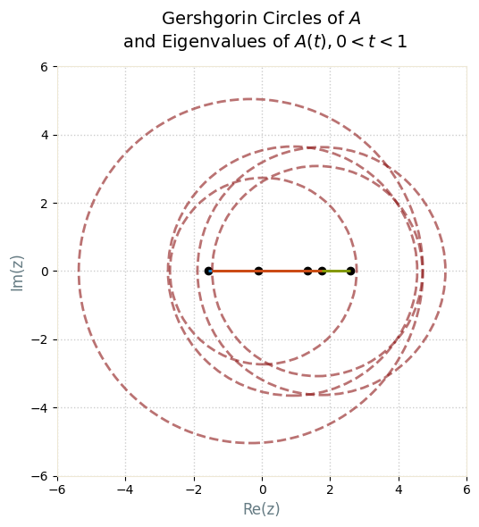
We can see that as we vary $$t$$, we are essentially observing the locus of eigenvalues of $$A(t)$$, all of them bounded by the Geršgorin’s discs. This immediately reminds one of the roots of a different polynomial: $$p_K(z) = D(s) + KN(s)$$. This is the root locus of an open-loop transfer function $$N(s)/D(s)$$ with closed-loop feedback gain $$K$$. That is, the locus of all roots of $$p_K(s)$$ as $$K$$ varies unbounded. While this is not a homotopy at all, Geršgorin’s discs play a role similar to the root locus: they bound and structure the possible trajectories, though they don’t give the exact path. While the discs provide set-based boundaries, the root locus provides geometric trajectories of the poles.

So the homotopy proof for eigenvalues is essentially a root locus argument for matrix eigenvalues, where the discs act like root-locus constraints, and homotopy invariance formalizes the preservation of eigenvalue counts in each region.

And yes, since $$\sum_{n=1}^\infty 1/n^2 = \pi^2/6$$ as the Basel problem the matrix up top is positive due to Geršgorin’s discs and being diagonally dominant :)

Afterword

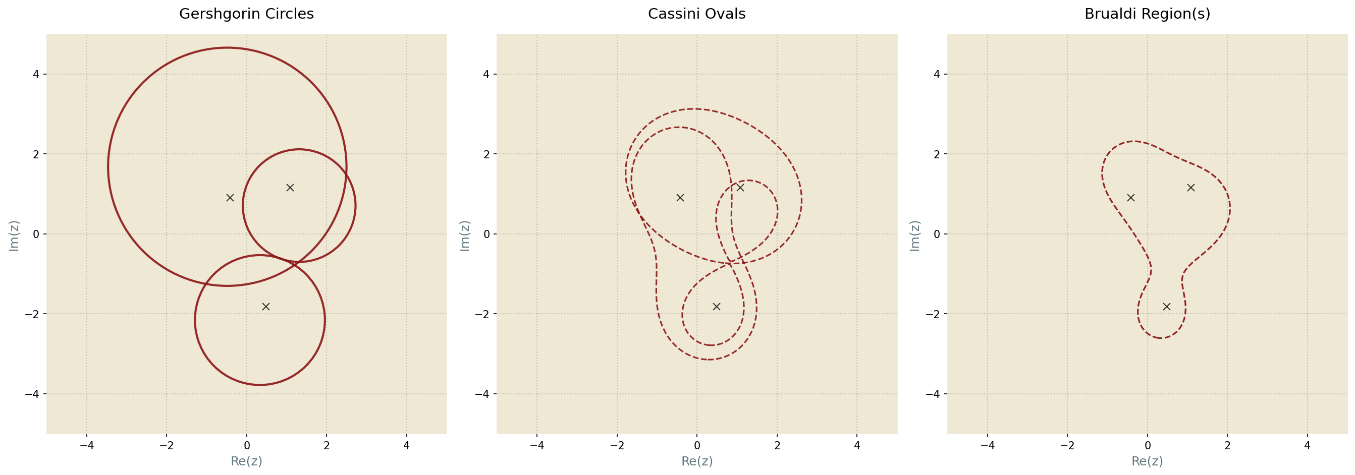
I recently learned about an interesting generalization of Geršgorin’s discs, called Brauer’s Cassini ovals. These are defined as $$\{z\in\mathbb{C}: |z-a_{ii}|\cdot|z-a_{jj}|\leq r_i r_j\}$$. These provide even tighter set enclosure for the eigenvalues using 2 rows at a time, as shown in the figure below.

Of course, even higher order generalizations exist, hence the curious field of eigenvalue localization using ever so sharp set boundaries! One such generalization are called Brualdi’s regions¹, which provide even sharper bounds for eigenvalues based on the matrix entries.

This article is a part of a side quest where I try to find amusing (at least to me!) applications of concepts form one engineering/mathematical field to another.

Written with StackEdit.